Semi-supervised image classification via Temporal Ensembling
Hi there ! This post aims to explain and provide implementation details on Temporal Ensembling, a semi-supervised method for image classification.
I will assume that you know the basics of Machine Learning and also a bit about neural networks.
Are you familiar with regularization, dropout, softmax, or stochastic gradient descent ?
If you don’t, I highly recommend going through some lectures of the Stanford course Convolutional Neural Networks for Visual Recognition, which, though vision-flavored, is an insanely good resource to get started in Machine Learning.
A few words on semi-supervised learning
Semi-supervised learning is an important subfield of Machine Learning.
It encompasses the techniques one can use when having both unlabeled data (usually a lot) and labeled data (usually a lot less). In that setting, unlabeled data can be used to improve model performance and generalization.
Labeled data is a scarce resource. Generally speaking, the whole labelling process is costly and needs active monitoring to avoid assessment flaws. Reliably performing semi-supervised solutions could have a huge impact on industries whose data is mostly untapped, like healthcare or automated driving.
In our case, we want to see how far we can get on MNIST using only 100 labels out of the 60000 available. Let’s go !
Temporal Ensembling
Temporal Ensembling was introduced by Timo Aila and Samuel Laine (both from NVIDIA) in 2016.
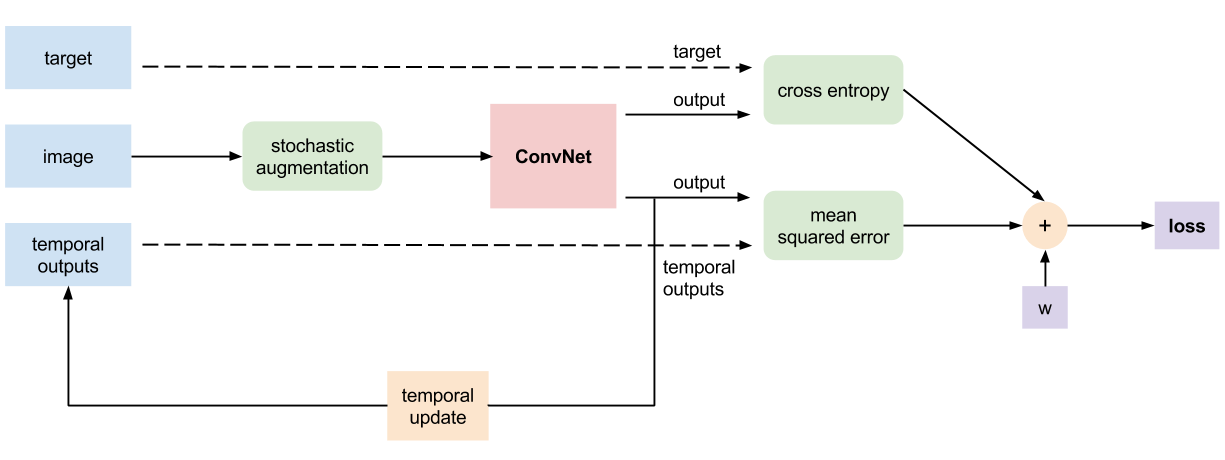
It comes from a relatively simple idea : that we can use an ensemble of the previous outputs of a neural network as an unsupervised target.
This is called self-ensembling.
In practice it means that they compare the network current outputs (post-softmax) to a weighted sum of all its previous outputs. Previous outputs are gathered during training : in an epoch, each input is seen once and its corresponding output is memorized to serve as comparison later.
Why does it work ?
If supervised learning was a cake, no doubt that labels would be the cherries on top that make it so good. Well, semi-supervised learning is the exact same cake except it has many less cherries by default, so one needs to fake them. In other words, one needs to have a proxy for the true label of the unlabeled samples. It does not need to be a 100% faithful reflection of the label : the proxy’s function is to guide the network in the right direction. If you pause the training process and consider the current model prediction, it is very likely that an ensemble of all previous predictions is more accurate and hints towards the true label. Hence, the self-ensemble is a handy label proxy that they use as a substitute for the missing cherries.
To make the ensembled predictions more diverse, they augment the inputs using gaussian noise, and add dropout regularization. Doing that, they give an incentive to the network not to completely shift its prediction for a slightly different version of the same input, which is a desirable property anyway ! To put it another way, injecting noise helps the network learn noise-invariant features.
Since they use dropout, their ensemble can be seen as an implicit mix of the predictions of all sub-networks they leveraged dropping neurons randomly in the network.
Their results are impressive : they get state-of-the-art performance on CIFAR10, CIFAR100 and SVHN (a house numbers recognition dataset), often by a large margin. For instance, they reduce the error rate from 18% to 5% on SVHN with 500 labels and from 18% to 12% on CIFAR10 with 4000 labels ! In both cases, the seed variance is smaller by an order of magnitude compared to the previous best method (that uses GANs in a semi-supervised way).
Without further ado, let’s try it ourselves !
The code
The code is in PyTorch. I’ll walk you through the most important parts of it, otherwise you can access the full code on GitHub.
The model
We will be using a very simple ConvNet with 2 conv layers, ReLU activations and one fully connected layer on top.
class CNN(nn.Module):

    def __init__(self, std):
        super(CNN, self).__init__()
        self.std   = std
        self.gn    = GaussianNoise(std=self.std)
        self.act   = nn.ReLU()
        self.drop  = nn.Dropout(0.5)
        self.conv1 = weight_norm(nn.Conv2d(1, 16, 3, padding=1))
        self.conv2 = weight_norm(nn.Conv2d(16, 32, 3, padding=1))
        self.mp    = nn.MaxPool2d(3, stride=2, padding=1)
        self.fc    = nn.Linear(32 * 7 * 7, 10)

    def forward(self, x):
        if self.training:
            x = self.gn(x)
        x = self.act(self.mp(self.conv1(x)))
        x = self.act(self.mp(self.conv2(x)))
        x = x.view(-1, 32 * 7 * 7)
        x = self.drop(x)
        x = self.fc(x)
        return x
Gaussian noise (centered) is applied to the inputs. The standard deviation chosen defines the aggressiveness of the transformation we want to teach the network to be robust to.
class GaussianNoise(nn.Module):

    def __init__(self, shape=(100, 1, 28, 28), std=0.05):
        super(GaussianNoise, self).__init__()
        self.noise = Variable(torch.zeros(shape).cuda())
        self.std = std

    def forward(self, x):
        c = x.shape[0]
        self.noise.data.normal_(0, std=self.std)
        return x + self.noise[:c]
Preprocessing
MNIST dataset can be loaded using the datasets module from torchvision.
We download the images, turn the numpy arrays into torch tensors, and apply pixel normalization.
def prepare_mnist():
    # normalize data
    m = (0.1307,)
    st = (0.3081,)
    normalize = tsfs.Normalize(m, st)

    # load train data
    train_dataset = dsts.MNIST(root='../data',
                               train=True,
                               transform=tsfs.Compose([tsfs.ToTensor(),
                                                       normalize]),
                               download=True)

    # load test data
    test_dataset = dsts.MNIST(root='../data',
                              train=False,
                              transform=tsfs.Compose([tsfs.ToTensor(),
                                                      normalize]))

    return train_dataset, test_dataset
The training loop
It starts like your standard PyTorch training loop : we retrieve the data, make data loaders (think generators for images and labels) and build the model.
# retrieve data
train_dataset, test_dataset = prepare_mnist()
ntrain = len(train_dataset)

# build model
model = CNN(std)
model.cuda()

# make data loaders
train_loader, test_loader = sample_train(train_dataset, test_dataset, batch_size,
                                         k, seed, shuffle_train=False)

# setup param optimization
optimizer = torch.optim.Adam(model.parameters(), lr=lr, betas=(0.9, 0.99))

# train
model.train()
losses = []
sup_losses = []
unsup_losses = []
best_loss = 20.
Now, a little bit more details about how to proceed with temporal ensembling.
We will be storing snapshot outputs in tensors. This is quite memory intensive but essential to compare the current outputs to the previous ones.
Z = torch.zeros(ntrain, n_classes).float().cuda()        # intermediate values
z = torch.zeros(ntrain, n_classes).float().cuda()        # temporal outputs
outputs = torch.zeros(ntrain, n_classes).float().cuda()  # current outputs
The loss function we use is a linear combination of the masked crossentropy and the mean square error between the current outputs (\(z_{i}\)) and the temporal outputs (\(\tilde{z}_{i}\)) :
\[l_{B}(z, \tilde{z}, y) = masked\_crossentropy(z, y) + w(t) * MSE(z, \tilde{z})\]The masked crossentropy takes only into account samples that possess a label. Calling \(B\) the set of minibatch indices, \(L\) the set of indices of labeled examples and \(C\) the amount of classes, it is expressed this way :
\[masked\_crossentropy(z, y) = - \frac{1}{\mid B \cap L \mid} \sum_{i \in (B \cap L)}{\log{z_{i}[y_{i}]}}\]and mean square error is calculated like this :
\[MSE(z, \tilde{z}) = \frac{1}{C \mid B \mid} \sum_{i \in B}{\mid \mid z_{i} - \tilde{z}_{i} \mid \mid ^{2}}\]The workaround to limit the crossentropy to the labeled samples is to set the label of the unlabeled images to -1 to create the mask :
def temporal_loss(out1, out2, w, labels):

    # MSE between current and temporal outputs
    def mse_loss(out1, out2):
        quad_diff = torch.sum((F.softmax(out1, dim=1) - F.softmax(out2, dim=1)) ** 2)
        return quad_diff / out1.data.nelement()

    def masked_crossentropy(out, labels):
        nbsup = len(torch.nonzero(labels >= 0))
        loss = F.cross_entropy(out, labels, size_average=False, ignore_index=-1)
        if nbsup != 0:
            loss = loss / nbsup
        return loss, nbsup

    sup_loss, nbsup = masked_crossentropy(out1, labels)
    unsup_loss = mse_loss(out1, out2)
    return sup_loss + w * unsup_loss, sup_loss, unsup_loss, nbsup
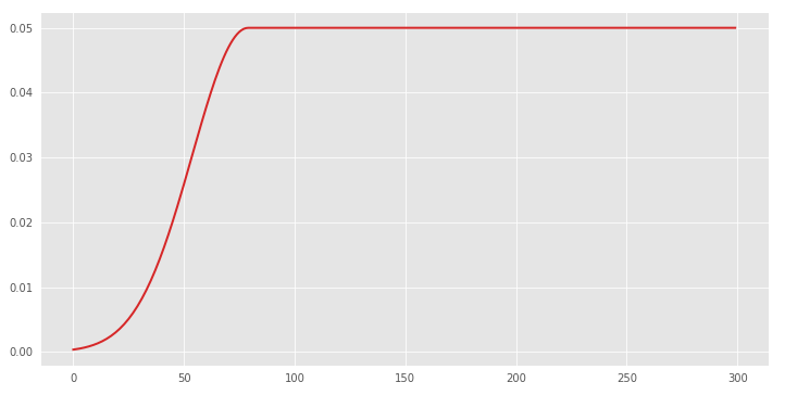
The unsupervised component is weighted by a function (\(w_{T}\)) that slowly ramps up. It is defined by the expression \(w_{T}(t) = \exp(-5(1 - \frac{t}{T})^{2})\) and has this shape :
Here’s the logic of our training loop :
for epoch in range(num_epochs):
    t = timer()

    # evaluate unsupervised cost weight
    w = weight_schedule(epoch, max_epochs, max_val, ramp_up_mult, k, n_samples)

    if (epoch + 1) % 10 == 0:
        print 'unsupervised loss weight : {}'.format(w)

    # turn it into a usable pytorch object
    w = torch.autograd.Variable(torch.FloatTensor([w]).cuda(), requires_grad=False)

    l = []
    supl = []
    unsupl = []
    for i, (images, labels) in enumerate(train_loader):
        images = Variable(images.cuda())
        labels = Variable(labels.cuda(), requires_grad=False)

        # get output and calculate loss
        optimizer.zero_grad()
        out = model(images)
        zcomp = Variable(z[i * batch_size: (i + 1) * batch_size], requires_grad=False)
        loss, suploss, unsuploss, nbsup = temporal_loss(out, zcomp, w, labels)

        # save outputs and losses
        outputs[i * batch_size: (i + 1) * batch_size] = out.data.clone()
        l.append(loss.data[0])
        supl.append(nbsup * suploss.data[0])
        unsupl.append(unsuploss.data[0])

        # backprop
        loss.backward()
        optimizer.step()

        # print loss
        if (epoch + 1) % 10 == 0:
            if i + 1 == 2 * c:
                print ('Epoch [%d/%d], Step [%d/%d], Loss: %.6f, Time (this epoch): %.2f s'
                       % (epoch + 1, num_epochs, i + 1, len(train_dataset) // batch_size, np.mean(l), timer() - t))
            elif (i + 1) % c == 0:
                print ('Epoch [%d/%d], Step [%d/%d], Loss: %.6f'
                       % (epoch + 1, num_epochs, i + 1, len(train_dataset) // batch_size, np.mean(l)))

    # update temporal ensemble
    Z = alpha * Z + (1. - alpha) * outputs
    z = Z * (1. / (1. - alpha ** (epoch + 1)))

    # handle metrics, losses, etc.
    eloss = np.mean(l)
    losses.append(eloss)
    sup_losses.append((1. / k) * np.sum(supl))  # divide by 1/k to obtain the mean supervised loss
    unsup_losses.append(np.mean(unsupl))

    # saving model
    if eloss < best_loss:
        best_loss = eloss
        torch.save({'state_dict': model.state_dict()}, 'model_best.pth.tar')
In each minibatch, we calculate the model output and the loss based on the previous outputs and the available labels.
After each epoch, we update the temporal outputs :
\[Z = \alpha Z + (1 - \alpha) z\]Since \(Z\) is initialized as a zero tensor, after the first epoch we have \(Z = (1 - \alpha) z\). We fix this startup bias this way :
\[\tilde{z} = \frac{Z}{1 - \alpha^{t}}\]In a nutshell, we compare the model outputs to an exponential moving average of the previous outputs, which gives greater weights to the most recent ones.
The test loop :
# test
model.eval()
acc = calc_metrics(model, test_loader)
if print_res:
    print 'Accuracy of the network on the 10000 test images: %.2f %%' % (acc)

# test best model
checkpoint = torch.load('model_best.pth.tar')
model.load_state_dict(checkpoint['state_dict'])
model.eval()
acc_best = calc_metrics(model, test_loader)
if print_res:
    print 'Accuracy of the network (best model) on the 10000 test images: %.2f %%' % (acc_best)

return acc, acc_best, losses, sup_losses, unsup_losses
The results
We train the model for 300 epochs, using a 0.002 learning rate and Adam as the optimizer, on a p2.xlarge Amazon AWS instance. The hyperparameters linked to temporal ensembling are those of the paper :
GLOB VARS
n_exp        = 5             # number of different seeds we try out
k            = 100           # labeled samples
MODEL VARS
drop         = 0.5           # dropout
std          = 0.15          # std of Gaussian noise
fm1          = 16            # number of feature maps in first conv layer
fm2          = 32            # number of feature maps in second conv layer
w_norm       = True
OPTIM VARS
lr           = 0.002
beta2        = 0.99          # second moment for Adam
num_epochs   = 300
batch_size   = 100
TEMP ENSEMBLING VARS
alpha        = 0.6           # ensembling momentum
data_norm    = channelwise   # image normalization
divide_by_bs = False         # whether we divide supervised cost by batch_size
Let’s have a look at the results :
RESULTS
best accuracy : 98.38
accuracy : 97.778 (+/- 0.627)
accs : [97.99, 98.13, 96.58, 97.81, 98.38]
Wow ! For a model as simple as the one we chose, just as advertised, we manage to get past 98% test accuracy, and even get 97.8% on average. To put things in perspective, training the same model the classic way on 100 images reaches only 88% accuracy. To the best of my knowledge, the state-of-the-art performance on this very task is 99.4% (Sajjadi et al.) and uses geometric augmentation.
The seed variance is also pretty fine, considering that we only use 100 labeled images randomly sampled from the dataset (which happens to have many low quality samples).
Here are the seed samples for our best model :
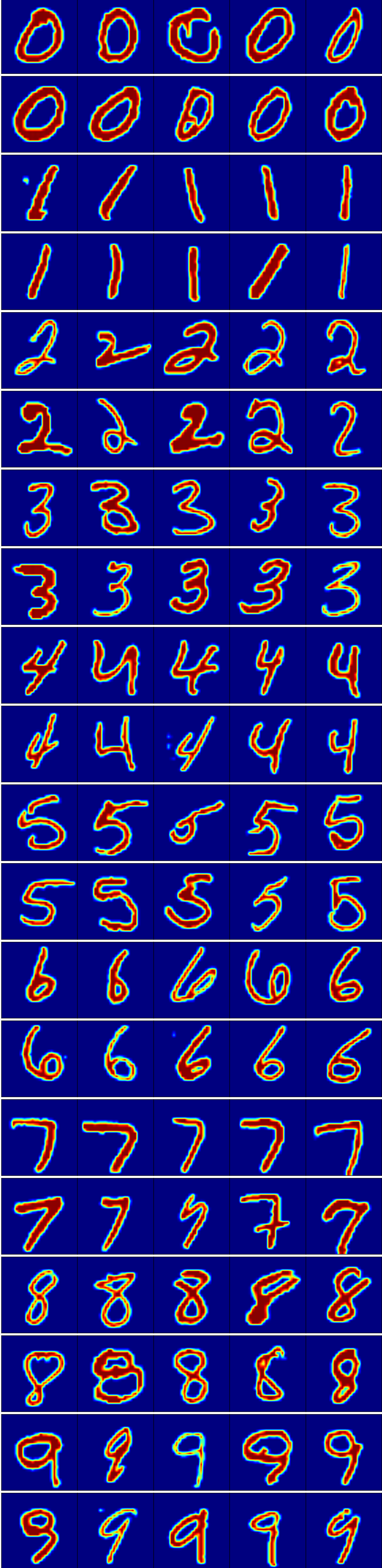
As you can see, the samples are far from perfect (sorry digits !).
In addition, with both criteria converging, the training dynamic looks great :
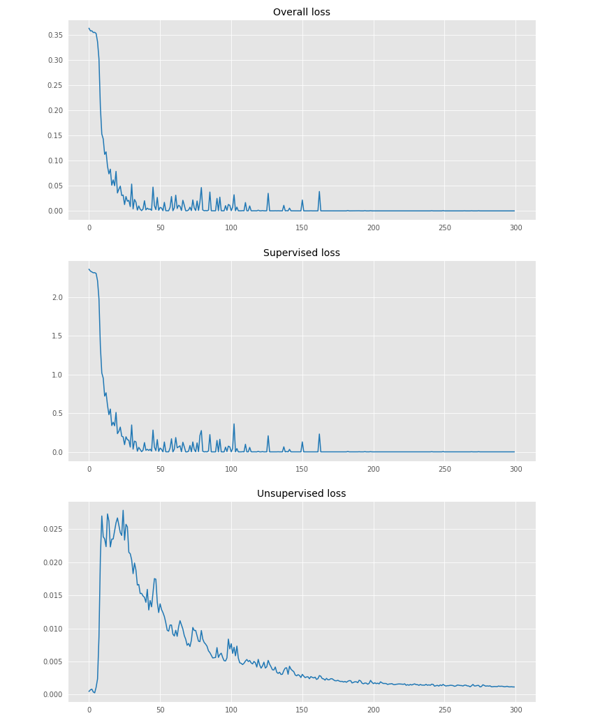
In the beginning, the supervised cost dominates clearly due to the slowly increasing weight of the unsupervised cost. As a result, the unsupervised cost first increases violently until its gradients start taking effect.
Though MNIST can be considered as a toy dataset by the actual Machine Learning standards, showing robust performance on a weakly-supervised setting is less trivial. It is a strong indicator that Temporal Ensembling is a solid approach to consider for semi-supervised learning.
A short disclaimer
In retrospect it’s always easy to make things look powerful or even magical (in particular in ML). For my part, I had to tweak a bit the algorithm to get there :
Using channelwise normalization
I found that using a channelwise instead of a pixelwise normalization during preprocessing gave consistently better results (1-2% accuracy).
Scaling supervised cost
In their code, the authors divide the sum of log probabilities (calculated on labeled samples) by the batchsize to calculate the masked crossentropy. I was puzzled by that choice and decided to try dividing by the amount of labeled samples in the batch instead. As a result, the supervised cost dominates more often, and the outcomes are slightly better and more stable.
Cursed local minima
Sometimes, the SGD got stuck in local minima where inference is as good as random. This is something the authors discuss in the article : “We have found it to be very important that the ramp-up of the unsupervised loss component is slow enough—otherwise, the network gets easily stuck in a degenerate solution where no meaningful classification of the data is obtained”.
Related work
I read some more recent papers exploring ideas intimely related to Temporal Ensembling :
Basically, in a fully supervised setting, instead of using the temporal ensemble as a target for self-ensembling, you use it as a stronger predictor. Like classic ensembling but free of charge ! Add cyclic learning rates, and you get impressive performance.
I love this paper. The idea is crazy simple : use linear combinations of pairs of samples (and the same for their labels) to create data augmented samples. It even works on images - who would have thought ? The link between both papers lies in the shaping of the decision function : when temporal ensembling imposes flatness near all data points via MSE, mixup imposes smoothness between data points via linear combinations.
This blog post reformulates mixup in a smart way, making it applicable in a semi-supervised setting !
I believe that we will hear more on shape constraints for decision functions in 2018.
Going further
I did not try these myself yet, feel free to experiment !
Adding data augmentation
Adding transformations on images is a go-to trick to improve ConvNets performance on vision tasks. It forces the network to find features that are robust to these transformations : in practice, augmenting inputs with rotations makes the network rotation-invariant. Of course, these transformations must not change the outcome of the prediction. In our case, they also extend the vicinity on which we incentive our network to stay coherent on in the input space.
This should be an easy way to get closer to 99% accuracy in my opinion.
The usual performance tricks
Here are some things you can try to get more faithful to the original implementation and hopefully improve performance :
- increase model capacity going wider and deeper
- replace ReLUs with leaky ReLUs
- add mean-only batch norm on top of weight normalization
See the paper (appendix A) for details.
Ensembling weights instead of outputs
Published at NIPS 2017, the paper Mean Teachers are Better Role Models: Weight-averaged Consistency Targets Improve Semi-Supervised Deep Learning Results provides an even more polished solution to the semi-supervised problem for images.
In a nutshell, Mean Teacher keeps a weighted sum of the snapshot model weights (aka the Teacher) instead of model outputs, and pushes the prediction of the current network (aka the Student) towards the Teacher via crossentropy.
If you want to dive deeper, check this excellent post by Curious AI.
Conclusion
Self-ensembling via temporal ensembling is a cheap but powerful way to squeeze more performance out of a ConvNet, whether you have unlabeled samples or not.
Don’t be scared by the additional hyperparameters : many of them work right off the bat with the values provided in the article.
And if your pipeline involves data augmentation - well, it could even work better.
Many thanks to DreamQuark for giving me the opportunity to share openly about a subject that I explored during my work as a research engineer. If you’re interested by this kind of research, do check their open positions, the team is great !
The code is available on GitHub.
Thanks for your neural attention !